*FNO를 위한 논문 리뷰 글입니다! 궁금하신 점은 댓글로 남겨주세요!
FNO paper: [2010.08895] Fourier Neural Operator for Parametric Partial Differential Equations (arxiv.org)
Fourier Neural Operator for Parametric Partial Differential Equations
The classical development of neural networks has primarily focused on learning mappings between finite-dimensional Euclidean spaces. Recently, this has been generalized to neural operators that learn mappings between function spaces. For partial differenti
arxiv.org
FNO github: GitHub - khassibi/fourier-neural-operator
GitHub - khassibi/fourier-neural-operator
Contribute to khassibi/fourier-neural-operator development by creating an account on GitHub.
github.com
Contents
Simple Introduction

'나비에 스토크스 방정식'을 혹시 들어보셨나요?
해당 방정식은 유체의 흐름과 이동에 대해서 설명하는 수식입니다..!
오늘날, 여러 연구들은 나비에 스토크스와 같은 유체의 흐름을 이해하는 물리 현상을 AI로 풀고자 노력중입니다!
이전에는 전산 유체역학이라는 분야에서 많이 다뤘죠!
21세기, 비행기나 자동차에 유체흐름에 관한 저항을 계산하는 걸 우리는 흔히 볼 수 있습니다.
이것이 전부, 유체의 흐름을 설명하는 방정식을 활용해서 컴퓨터가 계산하게 되는데 trivial solution을 찾진 못해서 근사해를 활용합니다.
이런 유체 흐름을 해석하는 곳에 수학적인 기법인 '푸리에 변환'과 AI를 같이 사용한 FNO을 소개하고자 합니다!
[참고] Navier-Stokes Equation에 대한 간단한 설명

저는 나비에 스토크스 방정식을 이해하기 위해서
'An Introduction to Computational Fluid Dynamic' 책을 참고하여 공부했습니다!
물론 FNO를 이해하는데 navier-stokes equation을 이해할 필요성은 없지만, 관심있는 분들은 위의 책에서 (2.1~2.4)까지 공부해보시기를 추천드립니다! (저는 공부하는데 한 6주?걸 것 같네요..물리 노베이스라서..ㅠ)
간단하게 (2.34~2.35) 수식을 설명드리면 아래와 같습니다.
(Navier-stokes equation를 활용한 방정식들)
2.34 equation: x,y,z에 대한 momentum 수식입니다(u,v,w가 각각의 symbol).
위에서 보이는 좌변의 p는 density이고, 우변의 p는 pressure입니다.
해당 수식을 전개하기 위해, 유체 volume 안에서 일어나는 mass conversation, heat conduction, viscous term(점성) 등등이 모두 고려되었습니다.
2.35 equation: (2.34)와 거의 비슷한데, 단지 해당 수식은 internal energy에 대한 navier-stokes equation 입니다.

사실 naiver-stokes equation에서 중요한 포인트는 다음이라고 생각합니다. (개인생각)
- 유체의 흐름과 성질을 설명할 때 여러 관점에서 설명이 가능함.
-> 예를 든다면, mass conversation, energy, momentum
- Mass conversation은 시간에 대한 고려가 필요없는 Eulerian approach로 설명이 가능함.
- 그러나 energy나 momentum의 경우 시간에 따른 fluid particle의 특성이 고려되어서 해석이 되어야 하므로, Lagrangian approach로 설명해야함.
- 이러한 두 해석차이를 메꿔주기 위해 material derivative를 활용할 수 있음.
-> (2.34, 2.35 equation의 좌변에 해당하는 방정식)
- 즉, 나비에-스토크스 방정식은 유체 유동을 설명하기 위해 material derivative를 도입하여서 수식을 전개함.
(저는 여기까지 이해한 것이 한계였습니다..ㅎㅎ)
Fourier Neural Operator
What is Fourier Transform?

'푸리에 변환'은 다음과 같다.
-> 임의의 입력함수(빨간색 그래프)가 들어왔을 때, sin-cos으로 구성된 주기함수의 합으로 분해하여 표현할 수 있다.
위에서 보이는 이미지의, 파란색 막대그래프는 각 주기함수들의 강도를 나타낸다.
또한 푸리에 변환의 특성은 다음과 같다
- 비주기 신호에 대해서 수행할 때, 이산적인 신호를 연속적으로 표현한다.
- 즉, 시간이 무한으로 흘러간다고 가정이 있다. (비주기 신호라는 것은 주기가 무한대라고 생각)
- 푸리에 급수에서 파생되어, 결과적으로 분해된 주기함수들의 합은 적분으로 표현된다.
FNO에서 주의해야할 점은, 우리의 데이터는 무한대가 아니기 때문에 discret fourier transform을 다루게 된다는 것이다!
<아래 블로그에서, fourier transform에 대한 유도과정을 살펴볼 수 있습니다!>


[참고자료 2]:
퓨리에 변환[Fourier transform, FT] (soojin7897.github.io)
푸리에 변환(Fourier transform) (tistory.com)
Fourier Neural Operator (FNO)

Iterative updates

논문에서는 첫번째 definition으로 'Iterative updates'를 보여준다.
해당 수식은, 논문의 figure2에서 fourier layer를 나타내는 것 같다.
K는 fourier transform을 적용하는 kernel 부분을 나타내는 것이고, W는 Vt(x)에 대한 linear transformation, sigma는 non-linear activation function이다.
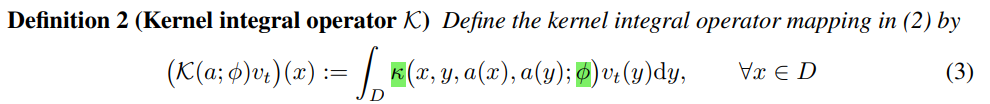
Fourier Intergral Operator K

위의 논문에서 나온 symbol을 정의해보자.
- D는 bounded인 dataset.
- A는 input에 해당하는 dataset.
- U는 output에 해당하는 dataset.

더불어서 convolution theorem이 무엇인지도 간단히 언급하겠습니다!
Fourier transform에서 이루어지는 합성곱 연산은, 단순하게 fourier transform을 적용한 각각의 함수의 곱셈과 같다는 의미입니다!
[참고자료(증명)]: [ Signal ]푸리에 변환과 합성곱의 관계(Convolution Theorem) (tistory.com)

위의 내용들을 간단히 나타내면 아래와 같습니다!
- 일단, kernel function (equation 3)을 보면 우리가 훈련시켜야 할 k라는 kernel이 a() 함수에 대해 의존성이 있다는 것을 알 수 있다.
- 여기서 k는 data로부터 학습해야할 kernel function을 의미합니다.
- 논문의 저자들은, a()라는 의존성을 없애고 단순하게 k(x,y)=k(x-y)라고 표현하였다. (수학적으로 왜 그런지는 모르겠음)
- 결과적으로 equation (3)는 단순한 k(x-y)와 v(y) 간의 convolution operator가 된다.
- 위와 같이 표현할 수 있는 equation (3)을 fourier transform과 convolution theorem 성질에 의해서 표현하면, equation (4)가 된다. (
-> 즉, 기존에 정의되던 kernel intergral operator mapping 함수를 fourier transform을 활용해서 재표현한 것이다.
-> 여기서, kernel function에 대한 fourier transform은 딥러닝이 학습해야하는 요소이므로 간단하게 R이라는 parameters로 표현한다.
또한, 우리는 컴퓨터 상에서 연산을 하는 것이기 때문에 어쩔 수 없이 discrete representation을 고려해야한다.
따라서, fourier transform을 적용한 후 나온 fourier series의 최대값을 설정하여 자른다.
+) 추가적으로, 논문의 저자들은 아래 부분에 Fourier Transform을 더 효율적으로 할 수 있는 Fast FT에 대해서도 언급하고 있는데 관심이 있다면 살펴보기를 바란다..!
Simple Code
# FNO 1-dimension에 대한 code.
## https://github.com/khassibi/fourier-neural-operator/blob/main/fourier_1d.py
class FNO1d(nn.Module):
    def __init__(self, modes, width):
        super(FNO1d, self).__init__()

        """
        The overall network. It contains 4 layers of the Fourier layer.
        1. Lift the input to the desire channel dimension by self.fc0 .
        2. 4 layers of the integral operators u' = (W + K)(u).
            W defined by self.w; K defined by self.conv .
        3. Project from the channel space to the output space by self.fc1 and self.fc2 .

        input: the solution of the initial condition and location (a(x), x)
        input shape: (batchsize, x=s, c=2)
        output: the solution of a later timestep
        output shape: (batchsize, x=s, c=1)
        """

        # default value 정의
        self.modes1 = modes
        self.width = width
        self.padding = 2 # pad the domain if input is non-periodic

        # FNO의 figure에서 P에 해당하는 값.
        self.fc0 = nn.Linear(2, self.width) # input channel is 2: (a(x), x)

        # 각각의 conv-w가 fourier layer
        self.conv0 = SpectralConv1d(self.width, self.width, self.modes1)
        self.conv1 = SpectralConv1d(self.width, self.width, self.modes1)
        self.conv2 = SpectralConv1d(self.width, self.width, self.modes1)
        self.conv3 = SpectralConv1d(self.width, self.width, self.modes1)
        self.w0 = nn.Conv1d(self.width, self.width, 1)
        self.w1 = nn.Conv1d(self.width, self.width, 1)
        self.w2 = nn.Conv1d(self.width, self.width, 1)
        self.w3 = nn.Conv1d(self.width, self.width, 1)

        # FNO의 figure2에서 Q에 해당하는 값.
        self.fc1 = nn.Linear(self.width, 128)
        self.fc2 = nn.Linear(128, 1)

    def forward(self, x):
        grid = self.get_grid(x.shape, x.device) # grid 생성.
        x = torch.cat((x, grid), dim=-1) # (batch, size_x, 2)
        x = self.fc0(x)
        x = x.permute(0, 2, 1)
        # x = F.pad(x, [0,self.padding]) # pad the domain if input is non-periodic

        x1 = self.conv0(x)
        x2 = self.w0(x)
        x = x1 + x2
        x = F.gelu(x)

        x1 = self.conv1(x)
        x2 = self.w1(x)
        x = x1 + x2
        x = F.gelu(x)

        x1 = self.conv2(x)
        x2 = self.w2(x)
        x = x1 + x2
        x = F.gelu(x)

        x1 = self.conv3(x)
        x2 = self.w3(x)
        x = x1 + x2

        # x = x[..., :-self.padding] # pad the domain if input is non-periodic
        x = x.permute(0, 2, 1)
        x = self.fc1(x)
        x = F.gelu(x)
        x = self.fc2(x)
        return x

    def get_grid(self, shape, device):
        batchsize, size_x = shape[0], shape[1]
        gridx = torch.tensor(np.linspace(0, 1, size_x), dtype=torch.float)
        gridx = gridx.reshape(1, size_x, 1).repeat([batchsize, 1, 1])
        return gridx.to(device)
-> 위의 부분이 바로, FNO 코드이다.
-> 데이터는 1d를 사용하는 것으로 가져왔다.
-> FNO 안의 fourier layer는 SpectralConv1d를 이용하는 것 같다.
# Fourier layer
class SpectralConv1d(nn.Module):
    def __init__(self, in_channels, out_channels, modes1):
        super(SpectralConv1d, self).__init__()

        """
        1D Fourier layer. It does FFT, linear transform, and Inverse FFT.
        """

        self.in_channels = in_channels
        self.out_channels = out_channels # FNO1d class의 width 값.
        self.modes1 = modes1  #Number of Fourier modes to multiply, at most floor(N/2) + 1

        self.scale = (1 / (in_channels*out_channels))
        # Kernel function에 해당하는 parameters 값. (trainable)
        self.weights1 = nn.Parameter(self.scale * torch.rand(in_channels, out_channels, self.modes1, dtype=torch.cfloat))

    # Complex multiplication
    def compl_mul1d(self, input, weights):
        # (batch, in_channel, x ), (in_channel, out_channel, x) -> (batch, out_channel, x)
        return torch.einsum("bix,iox->box", input, weights)

    def forward(self, x):
        batchsize = x.shape[0]
        #Compute Fourier coeffcients up to factor of e^(- something constant)
        x_ft = torch.fft.rfft(x) # fourier transform 적용하는 모듈!

        # Multiply relevant Fourier modes
        out_ft = torch.zeros(batchsize, self.out_channels, x.size(-1)//2 + 1,  device=x.device, dtype=torch.cfloat)
        out_ft[:, :, :self.modes1] = self.compl_mul1d(x_ft[:, :, :self.modes1], self.weights1)

        #Return to physical space
        x = torch.fft.irfft(out_ft, n=x.size(-1)) # Inverse fourier transform 적용.
        return x
-> 우리가 위의 equation (4)를 정의했던 것을 생각하면서 코드를 이해하면 쉽다!
-> 일단 self.weights1은 kernel function을 표현했던 parameters 값인 R이다.
-> 또한 pytorch에서 소개하는 코드로, torch.fft.rfft(x)를 통해 간단하게 fourier-transform을 적용한다.
-> torch.fft.rfft(x)로 나오는 x_ft는 수식에서 Vt(x)에 대한 fourier transform 값이다.
-> Equation (4)처럼, R과 x_ft를 서로 곱해준다.
-> 마지막으로, torch.fft.irfft를 적용해서 inverse fourier transform을 적용한다.
Result


- 이런 유체흐름을 AI로 학습하고, 시각화 하는 과정이 정말 매력있게 느껴진다..ㅎㅎ
- 2024.04.20 Kyujinpy 작성.


